Gibbs Sampler is an algorithm to build a Markov Chain having a given N-dimension limit distribution, exploring its conditional distribution.
The “Divide and Conquer” Intuition
Recap of Pain: In high-dimensional space (e.g., 100D), making a single acceptable proposal ($x_{new}$) with MH sampling is incredibly hard. It’s like trying to guess 100 coin flips correctly at once.
- While we can reduce multi-dimensional problems to one dimension via combination, when dimensions and state spaces are large, the resulting 1D state space becomes unmanageably huge.
Gibbs Strategy: Dimensionality Reduction (Divide and Conquer).
- We don’t change all dimensions at once.
- We update only one dimension at a time, treating the other 99 as constants (fixed).
Intuitive Analogy:
- MH Algorithm: Jumping randomly on a map like a helicopter.
- Gibbs Sampling: Walking on the streets of Manhattan, only moving East-West or North-South (Axis-aligned moves).
The MH Dilemma: High-Dimensional “Lottery”
Imagine you are doing a 100-dimensional sampling task (like generating a 10x10 pixel image, where each pixel is a dimension).
In Metropolis-Hastings (MH), you need a proposal distribution $Q$. If you try to update all 100 pixels at once:
- You are asking: “Hey, does this new combination of 100 numbers look like a reasonable image?”
- The probability of randomly guessing a “good point” in 100D space is as low as winning the lottery!
- Result: Your proposals are almost always rejected. Acceptance rate near 0, computer runs for days with no movement.
Gibbs Strategy: One Thing at a Time
Gibbs Sampling says: “Don’t be greedy. Since guessing 100 numbers is too hard, how about guessing just 1?”
Its logic:
- Lock dimensions 2 to 100 (pretend they are constants).
- Now, the question becomes: “Given everyone else is fixed, what is the best value for dimension 1?”
- This is a 1-dimensional problem! Too easy. We draw a number directly from this Conditional Distribution.
- Update dimension 1. Next, lock 1, 3…100, update dimension 2…
Core Philosophy: Break a complex $N$-dimensional problem into $N$ simple $1$-dimensional problems.
Math perspective: Convert Joint Distribution to Conditional Distributions.
Visual Intuition: Manhattan Walk
To visualize the trajectory, let’s compare MH and Gibbs on a 2D map. Assume we are climbing a mountain (Target $\pi$), peak is at top-right.
🚁 MH Algorithm: Helicopter Jump
- Action: Disregards terrain, throws a probe in a random direction (diagonal, far).
- Trajectory: Can move at any angle.
- Cost: If it lands on a cliff (low prob), it bounces back (Rejected).
🚶 Gibbs Sampling: Manhattan Walk
- Action: Imagine walking in Manhattan’s grid city. You can’t walk through walls or diagonally. You follow streets (axes).
- Trajectory:
- Move along X-axis (Update $x$, fixed $y$).
- Move along Y-axis (Update $y$, fixed $x$).
- Repeat.
- Feature: Trajectory is always orthogonal zig-zag, like climbing stairs.
Why is it Easy? (Slicing Thought)
You might ask: “Just changing direction, why no rejection needed?”
Imagine a 2D Normal distribution (like a hill). Each step of Gibbs is actually “Slicing” the hill.
- When you fix $y=5$, you slice the hill horizontally at $y=5$.
- The cross-section is a 1D curve.
- Gibbs says: “Please sample directly from this 1D curve.”
- Since you sample directly from the valid slice, the result is always valid. Acceptance Rate = 100%!
Mathematical Principles
Joint Distribution Equivalent to All “Full Conditionals”
Usually we think: Joint Distribution $P(x_1, \dots, x_n)$ holds all info. From it, deriving marginals or conditionals is easy. But the reverse isn’t intuitive: If I give you all “Full Conditionals” $P(x_i | x_{-i})$, can you uniquely reconstruct the original Joint Distribution?
Answer: Yes, under a condition (Positivity Assumption). This is Brook’s Lemma.
Proof
Step 1: Joint $\Rightarrow$ Conditionals (Easy)
This is just definition.
$$ P(x_i | x_{-i}) = \frac{P(x_1, \dots, x_n)}{P(x_{-i})} = \frac{P(x_1, \dots, x_n)}{\int P(x_1, \dots, x_n) dx_i} $$Obviously, given Joint, Conditionals are determined.
Step 2: Conditionals $\Rightarrow$ Joint (Hard: Brook’s Lemma)
This is the core of Gibbs. Without this, we wouldn’t know if sampling conditionals converges to the correct joint.
We need to prove: Full Conditionals uniquely determine Joint Distribution (up to a constant).
Let’s use Bivariate (2D) case ($x, y$).
- Goal: Find expression for $\frac{P(x, y)}{P(x_0, y_0)}$, where $(x_0, y_0)$ is an arbitrary reference point.
- Identity: Break ratio into two steps (via $(x_0, y)$): $$\frac{P(x, y)}{P(x_0, y_0)} = \frac{P(x, y)}{P(x_0, y)} \cdot \frac{P(x_0, y)}{P(x_0, y_0)}$$
- Expand Term 1 (Bayes): $P(x, y) = P(x | y) P(y)$. $$\frac{P(x, y)}{P(x_0, y)} = \frac{P(x | y) \cancel{P(y)}}{P(x_0 | y) \cancel{P(y)}} = \frac{P(x | y)}{P(x_0 | y)}$$ See! Marginal $P(y)$ cancels! Only conditionals remain.
- Expand Term 2: $P(x_0, y) = P(y | x_0) P(x_0)$. $$\frac{P(x_0, y)}{P(x_0, y_0)} = \frac{P(y | x_0) \cancel{P(x_0)}}{P(y_0 | x_0) \cancel{P(x_0)}} = \frac{P(y | x_0)}{P(y_0 | x_0)}$$ Marginal $P(x_0)$ cancels too!
- Combine (Brook’s Lemma for 2D): $$P(x, y) \propto \frac{P(x | y)}{P(x_0 | y)} \cdot \frac{P(y | x_0)}{P(y_0 | x_0)}$$
Conclusion: The RHS contains only conditional distributions. Thus, knowing $P(x|y)$ and $P(y|x)$ uniquely determines the shape of $P(x,y)$.
General N-Dim (Brook’s Lemma)
Ideally walking steps from $\mathbf{x}^0$ to $\mathbf{x}$: $(0,0,0) \to (x_1, 0, 0) \to (x_1, x_2, 0) \to (x_1, x_2, x_3)$.
Formula:
$$P(\mathbf{x}) \propto \prod_{i=1}^n \frac{P(x_i | x_1, \dots, x_{i-1}, x_{i+1}^0, \dots, x_n^0)}{P(x_i^0 | x_1, \dots, x_{i-1}, x_{i+1}^0, \dots, x_n^0)}$$Crucial Prerequisite: Positivity Condition
Did you spot a bug? We are dividing! Denominators like $P(x_0 | y)$ appear. If probability is 0 somewhere, dividing by 0 is illegal.
This is the Hammersley-Clifford Theorem requirement: Joint distribution must satisfy Positivity Assumption. i.e., For any $x_i$, if meaningful marginally, their combination $(x_1, \dots, x_n)$ must have prob > 0.
Counter-example: Chessboard where only white squares have prob=1, black=0.
- $P(x|y)$ tells you where white squares are in a row.
- But you can’t compare probability of white squares in different rows because “paths” are blocked by black squares (prob 0 abyss).
Why No Rejection? (Why Acceptance is 100%?)
Gibbs Sampling is essentially Metropolis-Hastings with acceptance rate $\alpha=1$.
Intuitive: Why no “Audit”?
- Metropolis (Blind Guess): You grab a shirt with eyes closed (Proposal $Q$). Open eyes, check fit ($\pi$). If bad, throw back (Reject). Blindness requires audit.
- Gibbs (Tailor-made): You go to a tailor. Tailor measures you (Fixed $x_{-i}$), makes shirt exactly to size (Sample from $P(x_i | x_{-i})$). Does this custom shirt need “audit”? No. It’s born valid.
Math Proof: MH Formula Cancellation
Assume variables $x, y$. Current: $(x, y)$
- Action: Update $x$, fix $y$.
- Gibbs Proposal: Sample new $x^*$ from full conditional. $$Q(\text{new} | \text{old}) = Q(x^*, y | x, y) = P(x^* | y)$$
Note: Depends only on $y$, not old $x$.
Reverse proposal:
$$Q(\text{old} | \text{new}) = Q(x, y | x^*, y) = P(x | y)$$Substitute into MH Acceptance:
$$\alpha = \frac{\pi(\text{new})}{\pi(\text{old})} \times \frac{Q(\text{old} | \text{new})}{Q(\text{new} | \text{old})}$$- Target $\pi$ is Joint $P(x, y)$. $$\text{Target Ratio} = \frac{P(x^*, y)}{P(x, y)}$$
- Proposal $Q$. $$\text{Proposal Ratio} = \frac{P(x | y)}{P(x^* | y)}$$
- Combine ($P(a,b) = P(a|b)P(b)$): $$A = \frac{P(x^*, y)}{P(x, y)} \times \frac{P(x | y)}{P(x^* | y)} = \frac{\mathbf{P(x^* | y)} \cdot \mathbf{P(y)}}{\mathbf{P(x | y)} \cdot \mathbf{P(y)}} \times \frac{\mathbf{P(x | y)}}{\mathbf{P(x^* | y)}}$$
- The Cancellation:
- $P(y)$: Cancels.
- $P(x^* | y)$ and $P(x | y)$: Cancel cross-wise.
- Result: $$A = 1$$
So $\alpha = 1$.
Algorithm Flow
To sample from $n$-dim joint $P(x_1, \dots, x_n)$.
- Initialization: Pick start $\mathbf{x}^{(0)}$.
- Iteration Loop ($t=1 \dots T$): Update each component sequentially. Updated values used immediately.
- Update Dim 1: Sample $x_1^{(t)} \sim P(x_1 \mid x_2^{(t-1)}, \dots, x_n^{(t-1)})$
- Update Dim 2: Sample $x_2^{(t)} \sim P(x_2 \mid x_1^{(t)}, x_3^{(t-1)}, \dots)$ …
- Update Dim $n$: Sample $x_n^{(t)} \sim P(x_n \mid x_1^{(t)}, \dots, x_{n-1}^{(t)})$
- Collect: $\mathbf{x}^{(t)}$ is a sample.
Update Strategies
- Systematic Scan: Order $1 \to 2 \to \dots \to n$. Most common.
- Random Scan: Randomly pick dimension $i$ to update. Easier for some proofs.
- Blocked Gibbs: Group correlated variables (e.g., $x_1, x_2$) and sample joint $P(x_1, x_2 | \dots)$. Solves slow mixing in correlated features.
Code Practice
Discrete: Bivariate System
Two variables $x, y \in \{0, 1\}$. Known joint probability table:
| x | y | P(x,y) |
|---|---|---|
| 0 | 0 | 0.1 |
| 0 | 1 | 0.4 |
| 1 | 0 | 0.3 |
| 1 | 1 | 0.2 |
Goal: Sample to match these frequencies using only local conditional rules.
Conditionals:
- Given $y$, $P(x|y)$:
- $y=0$: $P(x=0|0) = 0.1/(0.1+0.3) = 0.25$, $P(x=1|0)=0.75$
- $y=1$: $P(x=0|1) = 0.4/(0.4+0.2) \approx 0.67$, $P(x=1|1)=0.33$
- Given $x$, $P(y|x)$:
- $x=0$: $P(y=0|0) = 0.2$, $P(y=1|0)=0.8$
- $x=1$: $P(y=0|1) = 0.6$, $P(y=1|1)=0.4$
import numpy as np
import matplotlib.pyplot as plt

# 1. Conditionals
def sample_x_given_y(y):
    if y == 0:
        return np.random.choice([0, 1], p=[0.25, 0.75])
    else:
        return np.random.choice([0, 1], p=[0.67, 0.33])

def sample_y_given_x(x):
    if x == 0:
        return np.random.choice([0, 1], p=[0.2, 0.8])
    else:
        return np.random.choice([0, 1], p=[0.6, 0.4])

# 2. Gibbs Loop
def discrete_gibbs(n_iter):
    samples = []
    x, y = 0, 0  # Init

    for _ in range(n_iter):
        x = sample_x_given_y(y) # Update x
        y = sample_y_given_x(x) # Update y
        samples.append((x, y))

    return np.array(samples)

# 3. Run
n_iter = 10000
results = discrete_gibbs(n_iter)

# Frequency Analysis
unique, counts = np.unique(results, axis=0, return_counts=True)
frequencies = counts / n_iter

print("--- Discrete Gibbs Results ---")
for state, freq in zip(unique, frequencies):
    print(f"State {state}: Freq {freq:.4f}")

# Visualize first 50 steps
plt.figure(figsize=(6, 6))
plt.plot(results[:50, 0] + np.random.normal(0, 0.02, 50),
         results[:50, 1] + np.random.normal(0, 0.02, 50),
         'o-', alpha=0.5)
plt.xticks([0, 1])
plt.yticks([0, 1])
plt.title("Trace of First 50 Discrete Gibbs Steps\n(with small jitter for visibility)")
plt.xlabel("X state")
plt.ylabel("Y state")
plt.grid(True)
plt.show()
--- Discrete Gibbs Results ---
State [0 0]: Freq 0.1017
State [0 1]: Freq 0.4054
State [1 0]: Freq 0.2928
State [1 1]: Freq 0.2001
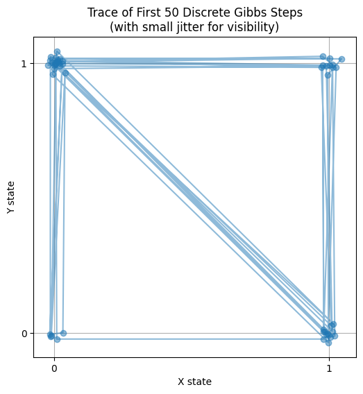
- Fast Convergence: Instantly locks to target propertions.
- Trajectory: Jumps between (0,0), (0,1), (1,0), (1,1) strictly along axes.
- Application: Core of Image Denoising (Ising) and NLP (LDA).
Continuous Example: Bivariate Normal Implementation
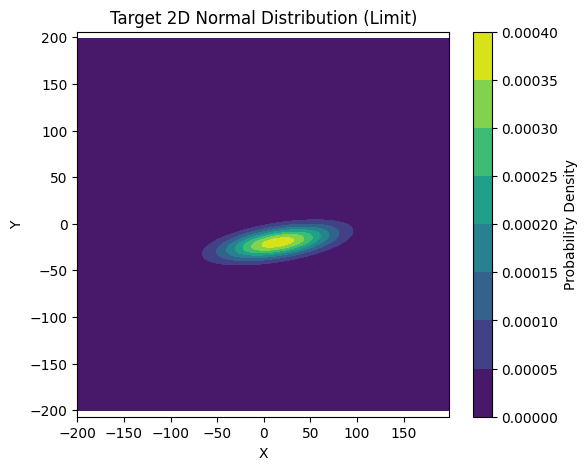
Our target is to sample a 2D vector $(x, y)$ from a Bivariate Normal Distribution, shaped like a tilted hill:
- Mean: $\mu_x = 15, \mu_y = -20$
- Center at $(15, -20)$.
- Standard Deviation: $\sigma_x = 40, \sigma_y = 12$
- $x$ is wide spread, $y$ is narrow.
- Correlation: $\rho = 0.5$
- Positive correlation, meaning as $x$ increases, $y$ tends to increase. The hill is tilted.
import numpy as np
import matplotlib.pyplot as plt
from scipy.stats import multivariate_normal

# --- 1. Define Distribution Parameters ---
mu_x, mu_y = 15, -20
s_x, s_y = 40, 12
r = 0.5  # Correlation coefficient

# Covariance Matrix Sigma = [[sx^2, r*sx*sy], [r*sx*sy, sy^2]]
cov_xy = r * s_x * s_y
Sigma = np.array([[s_x**2, cov_xy],
                  [cov_xy, s_y**2]])
Mean = np.array([mu_x, mu_y])

# --- 2. Create Grid for Plotting ---
x, y = np.mgrid[-200:200:1, -200:200:1]
pos = np.dstack((x, y))

# Calculate Theoretical PDF
rv = multivariate_normal(Mean, Sigma)
Z = rv.pdf(pos)

# --- 3. Visualize Target ---
plt.figure(figsize=(6, 5))
plt.contourf(x, y, Z, cmap='viridis')
plt.colorbar(label='Probability Density')
plt.title('Target 2D Normal Distribution (Limit)')
plt.xlabel('X')
plt.ylabel('Y')
plt.axis('equal')  # Keep aspect ratio
plt.show()
Comparing 4 Sampling Strategies
To understand the characteristics of Gibbs Sampling, we will compare it with different Metropolis strategies.
First, let’s define a plotting function to visualize the trajectory and mixing.
import matplotlib.pyplot as plt

def plot_trajectory(samples, title, method_name):
    """
    Plots 3 figures:
    1. 2D Density Map (Final Result)
    2. Trajectory of first 50 steps (Details)
    3. Trace Plot of X and Y (Mixing)
    """
    plt.figure(figsize=(15, 10))

    # Plot 1: Final Distribution
    plt.subplot2grid((2, 2), (0, 0))
    plt.hist2d(samples[:,0], samples[:,1], bins=50, cmap='viridis', density=True)
    plt.title(f'{title}\n(Final Distribution)')
    plt.axis('equal')

    # Plot 2: Trajectory (First 50 Steps)
    plt.subplot2grid((2, 2), (0, 1))
    # Background contours
    x, y = np.mgrid[-100:150:1, -100:50:1]
    pos = np.dstack((x, y))
    plt.contour(x, y, rv.pdf(pos), levels=5, cmap='Greys', alpha=0.3)

    # Path
    plt.plot(samples[:50, 0], samples[:50, 1], 'o-', markersize=4, linewidth=1, alpha=0.7, color='r')
    plt.scatter(samples[0, 0], samples[0, 1], color='k', s=50, label='Start', zorder=5)
    plt.title(f'{method_name} Path\n(First 50 Steps)')
    plt.xlabel('X')
    plt.ylabel('Y')
    plt.legend()
    plt.grid(True, linestyle='--', alpha=0.3)

    # Plot 3: Trace Plot (Mixing)
    plt.subplot2grid((2, 2), (1, 0), colspan=2)
    plt.plot(samples[:, 0], label='X', alpha=0.6, linewidth=0.5)
    plt.plot(samples[:, 1], label='Y', alpha=0.6, linewidth=0.5)
    plt.title(f'{method_name} Trace\n(Mixing)')
    plt.xlabel('Iteration')
    plt.legend()

    plt.tight_layout()
    plt.show()
Method 1: Standard Gibbs Sampler
If we want to sample directly (e.g., Rejection Sampling), we face a complex formula:
$$P(x, y) \propto \exp\left( -\frac{1}{2(1-\rho^2)} (x^2 - 2\rho xy + y^2) \right)$$With Gibbs, we use the conditional distributions, which are simple 1D Normals:
- Given $y$, $x \sim \mathcal{N}(\mu_{x|y}, \sigma_{x|y}^2)$
- Given $x$, $y \sim \mathcal{N}(\mu_{y|x}, \sigma_{y|x}^2)$
Intuition:
- Mean shift: If $x, y$ are positively correlated, knowing $y$ is large tells us $x$ is likely large.
- Variance reduction: High correlation reduces the conditional variance (uncertainty).
# ==========================================
# Method 1: Standard Gibbs Sampling
# ==========================================
print("Running Method 1: Standard Gibbs...")
n_iter = 100000
samples_gibbs = np.zeros((n_iter, 2))
curr = np.array([0.0, 0.0]) # Start

# Conditional Standard Deviations (fixed for Normal)
s_x_cond = s_x * np.sqrt(1 - r**2)
s_y_cond = s_y * np.sqrt(1 - r**2)

for i in range(n_iter):
    # 1. Update X (Fix Y)
    mu_x_cond = mu_x + r * (s_x / s_y) * (curr[1] - mu_y)
    curr[0] = np.random.normal(mu_x_cond, s_x_cond)

    # Note: Gibbs technically updates one by one. To plot perfect
    # orthogonal steps, we should record intermediate states.
    # Here we record after both updates for simplicity.

    # 2. Update Y (Fix X)
    mu_y_cond = mu_y + r * (s_y / s_x) * (curr[0] - mu_x)
    curr[1] = np.random.normal(mu_y_cond, s_y_cond)

    samples_gibbs[i] = curr

plot_trajectory(samples_gibbs, "Standard Gibbs", "Gibbs")
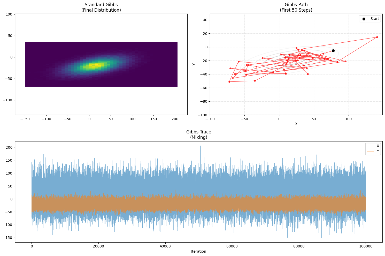
- Path Characteristic: Manhattan Walk.
- Logically, it moves strictly along axes (“Move X, then Move Y”).
- It navigates the tilted ellipse efficiently using conditional guidance.
- Acceptance Rate: 100%. No rejection.
Method 2: Gibbs via Metropolis (Metropolis-within-Gibbs)
What if we don’t know the exact formula for $P(x|y)$? Or if it’s too complex to sample directly? We can use Metropolis steps to simulate the conditional sampling.
- Principle:
- Update $x$: Fix $y$. Use Metropolis to propose a new $x$ and accept/reject it based on $P(x|y)$.
- Update $y$: Fix $x$. Use Metropolis to propose a new $y$.
- Pros: Generic. Works without analytical conditionals.
- Cons: Slower due to rejections.
# ==========================================
# Method 2: Gibbs via Metropolis
# ==========================================
print("Running Method 2: Gibbs via Metropolis...")
n_iter = 100000
samples_gm = np.zeros((n_iter, 2))
curr = np.array([0.0, 0.0])
prop_width = 100 # Large proposal width

for i in range(n_iter):
    # --- Update X (Metropolis) ---
    x_old, y_old = curr
    x_cand = np.random.uniform(x_old - prop_width, x_old + prop_width)

    # Acceptance ratio: P(x_new, y) / P(x_old, y)
    p_old = rv.pdf([x_old, y_old])
    p_new = rv.pdf([x_cand, y_old])
    alpha = min(1, p_new / p_old)
    if np.random.rand() < alpha:
        curr[0] = x_cand

    # --- Update Y (Metropolis) ---
    x_fixed, y_old = curr
    y_cand = np.random.uniform(y_old - prop_width, y_old + prop_width)

    alpha = min(1, rv.pdf([x_fixed, y_cand]) / rv.pdf([x_fixed, y_old]))
    if np.random.rand() < alpha:
        curr[1] = y_cand

    samples_gm[i] = curr

plot_trajectory(samples_gm, "Gibbs via Metropolis", "Gibbs-Metropolis")
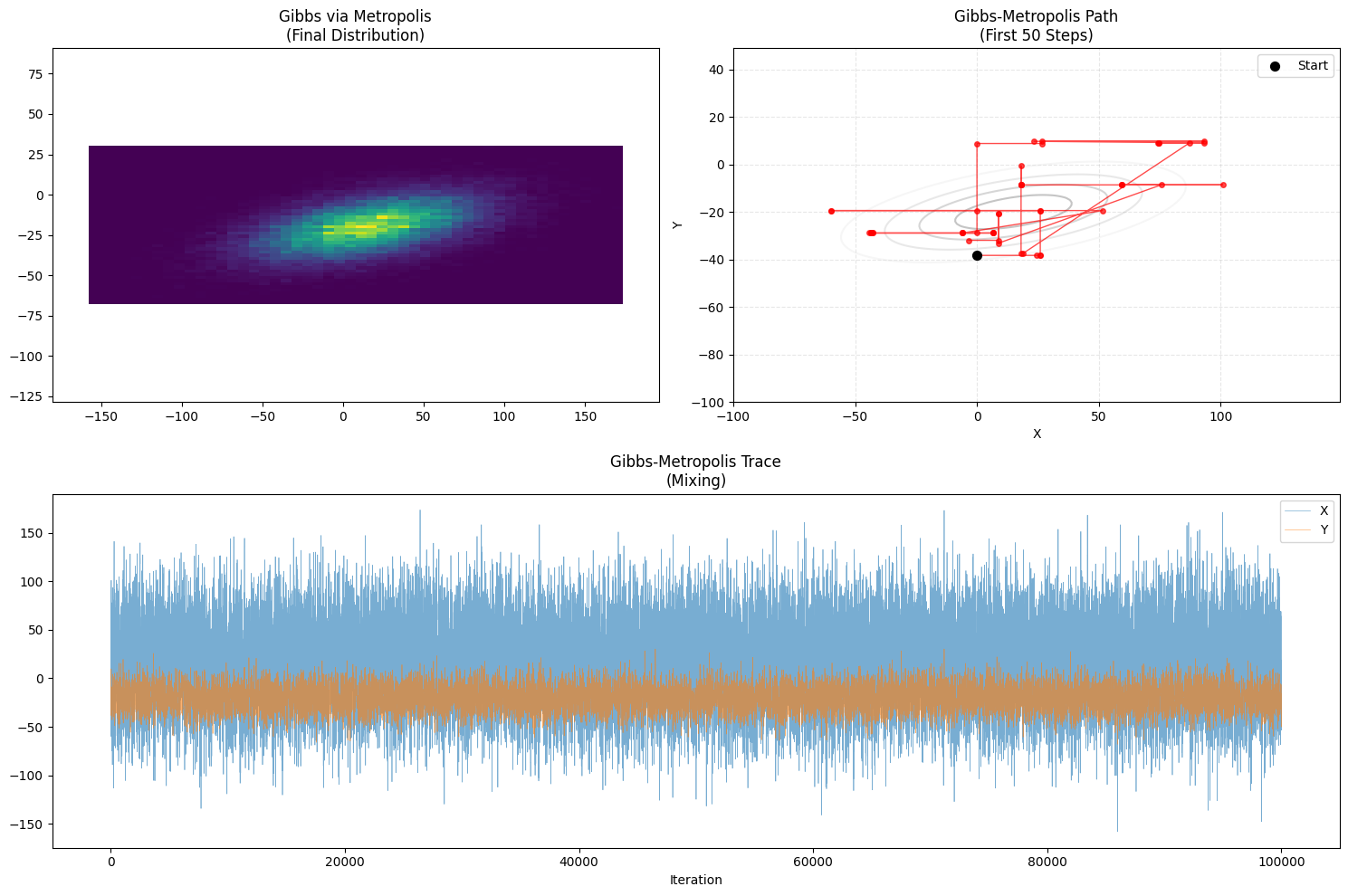
- Path Characteristic: Stuttering Manhattan Walk.
- Similar to Gibbs but with “pauses” (rejections) along the axes.
Method 3: Random Walk Metropolis (2D)
The “Standard” Metropolis. Update $(x, y)$ simultaneously.
- Principle: Propose $(x', y')$ by adding random noise to $(x, y)$. Accept/Reject based on joint ratio.
- Cons: In high dimensions or high correlation, guessing both $x$ and $y$ correctly at once is hard. Low acceptance.
# ==========================================
# Method 3: Random Walk Metropolis
# ==========================================
print("Running Method 3: Random Walk Metropolis...")
n_iter = 100000
samples_rw = np.zeros((n_iter, 2))
curr = np.array([0.0, 0.0])
sigma_prop = 10

for i in range(n_iter):
    proposal = curr + np.random.normal(0, sigma_prop, size=2)

    p_curr = rv.pdf(curr)
    p_prop = rv.pdf(proposal)

    alpha = min(1, p_prop / p_curr)
    if np.random.rand() < alpha:
        curr = proposal

    samples_rw[i] = curr

plot_trajectory(samples_rw, "Random Walk Metropolis", "RW-Metropolis")
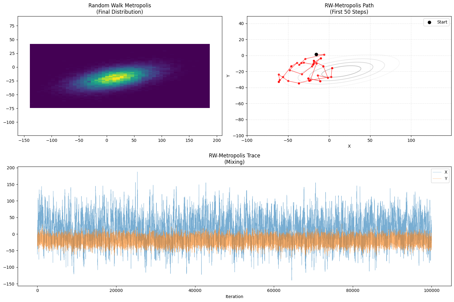
- Path Characteristic: Drunkard’s Walk.
- Moves in arbitrary directions.
- Often gets stuck or moves slowly compared to Gibbs in structured limits.
Method 4: Independent Metropolis Sampler
Propose new state $(x', y')$ completely independently of current state.
# ==========================================
# Method 4: Independent Metropolis
# ==========================================
print("Running Method 4: Independent Metropolis...")
n_iter = 100000
samples_ind = np.zeros((n_iter, 2))
curr = np.array([0.0, 0.0])
search_range = 200

for i in range(n_iter):
    proposal = np.random.uniform(-search_range, search_range, size=2)

    alpha = min(1, rv.pdf(proposal) / rv.pdf(curr))
    if np.random.rand() < alpha:
        curr = proposal

    samples_ind[i] = curr

plot_trajectory(samples_ind, "Independent Metropolis", "Indep-Metropolis")
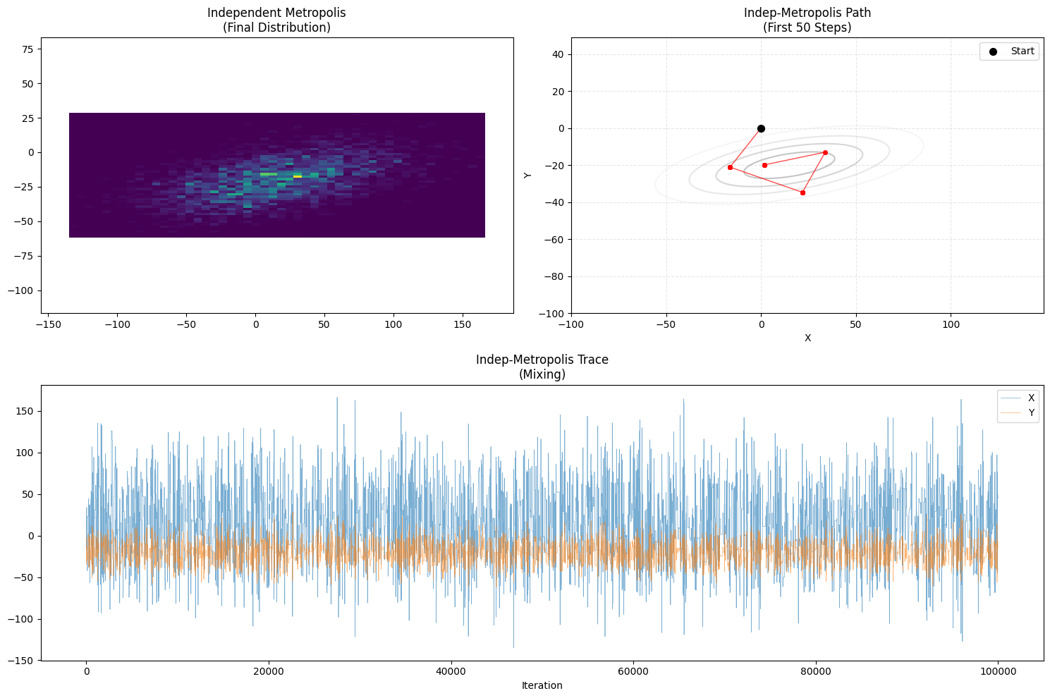
- Path Characteristic: Teleportation & Stagnation.
- Teleportation: Can jump from one end to another instantly (Great Mixing).
- Stagnation: Most proposals land in low-probability “wilderness” and are rejected. Long pauses.
Summary
| Method | Update Strategy | Acceptance | Best For |
|---|---|---|---|
| Standard Gibbs | Alternating x, y (Formula) | 100% | Conditional formula known (Gaussian, Beta…) |
| Metropolis-Gibbs | Alternating x, y (Guess) | Medium | Conditional formula unknown but want “divide & conquer” |
| Pure Metropolis | Simultaneous x, y | Low | Simple problems, or when conditionals are hard to derive |
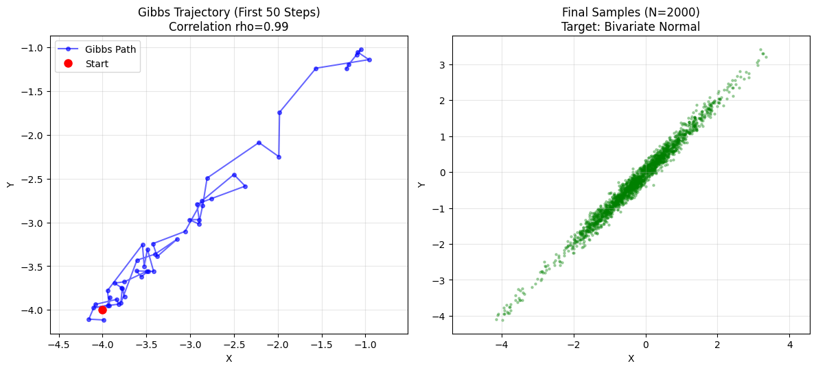
The Kryptonite: High Correlation
- Defect: 100% acceptance $\neq$ Efficiency.
- Scenario: High correlation ($\rho = 0.99$). Distribution is a thin canyon.
- Dilemma: Gibbs moves orthogonally. In a diagonal canyon, it must take tiny baby steps (staircase). Slow Mixing.
- Solution: Blocked Gibbs / Reparameterization.
import numpy as np
import matplotlib.pyplot as plt

# --- 1. Params ---
rhos = {0: 'No Corr', 0.99: 'High Corr'}
n_samples = 2000
start_x, start_y = -4.0, -4.0

# --- 2. Gibbs Sampler (Reusable) ---
def run_gibbs_sampler(n, rho, start_x, start_y):
    samples = np.zeros((n, 2))
    x, y = start_x, start_y
    cond_std = np.sqrt(1 - rho**2)

    for i in range(n):
        # A. Fix y, sample x
        x = np.random.normal(loc=rho * y, scale=cond_std)

        # B. Fix x, sample y (use new x)
        y = np.random.normal(loc=rho * x, scale=cond_std)

        samples[i] = [x, y]

    return samples

# Run
index = 1
for rho, rho_label in rhos.items():
    chain = run_gibbs_sampler(n_samples, rho, start_x, start_y)

    # --- 3. Viz ---
    plt.figure(figsize=(12, 10))

    # Trace
    plt.subplot(2, 2, index)
    plt.plot(chain[:50, 0], chain[:50, 1], 'o-', alpha=0.6, color='blue', markersize=4, label='Gibbs Path')
    plt.plot(start_x, start_y, 'ro', label='Start', markersize=8)
    plt.title(f"Gibbs Trajectory (First 50 Steps)\nCorrelation rho={rho}")
    plt.xlabel("X")
    plt.ylabel("Y")
    plt.legend()
    plt.grid(True, alpha=0.3)
    plt.axis('equal')
    index += 1

    # Scatter
    plt.subplot(2, 2, index)
    plt.scatter(chain[:, 0], chain[:, 1], s=5, alpha=0.3, color='green')
    plt.title(f"Final Samples (N={n_samples})\nTarget: Bivariate Normal")
    plt.xlabel("X")
    plt.ylabel("Y")
    plt.axis('equal')
    plt.grid(True, alpha=0.3)
    index += 1

plt.tight_layout()
plt.show()
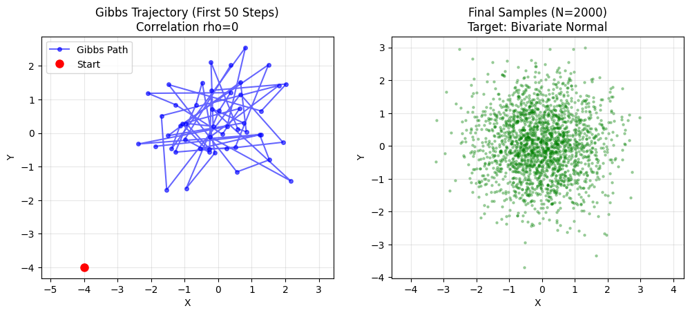
- rho = 0: Circle. Gibbs jumps freely. Fast mixing.
- rho = 0.99: Thin line. Gibbs takes tiny steps along diagonal. Slow convergence.
Scan to Share
微信扫一扫分享